Fisher Information
These are my personal study notes based on:
- Chapter 11 of Elements of Information Theory (Cover & Thomas, 2nd ed.)
- A Tutorial on Fisher Information (Ly et al., 2017)
All errors are my own. Please refer to the original texts for complete and authoritative treatment.
SETUP
Suppose we have a sample of data \(X_1, X_2, \dots, X_n\), each drawn i.i.d. from a certain parameterized probability function \(f(x_i; \theta)\). This whole sequence of data is also a random variable \(X^n = (X_1, \dots, X_n)\), and because of i.i.d., it follows the probability function
\[f(x^n; \theta) = \prod_{i=1}^{n} f(x_i; \theta). \tag{1}\]The parameter \(\theta\) is unknown, and usually it needs to be estimated from the raw data \(X^n\) or from a certain statistic \(T\) (e.g., the mean of the data). We want to know how much information the raw data or the statistic gives us about the parameter \(\theta.\) Fisher information \(J(\theta)\) quantifies exactly this.
SCORE FUNCTION
To calculate Fisher information, we first define a score function \(V\), which is a random variable that measures how sensitive the log-likelihood of \(X\) is to changes of the parameter \(\theta\):
\[V = \frac{\partial}{\partial \theta} \ln f(X; \theta).\]Note that \(X\) can be a sequence of data \(X^n\) with its density function given in Eq. (1).
DEFINITION OF FISHER INFORMATION
With the score function, Fisher information \(J(\theta)\) is defined as
\[\begin{aligned} J(\theta) &= \mathbb{E}_{X \sim f(x;\theta)} \left[ \left( \frac{\partial}{\partial \theta} \ln f(X; \theta) \right)^2 \right]\\ &= \int \left( \frac{\partial}{\partial \theta} \ln f(x; \theta) \right)^2 f(x;\theta) \, dx. \end{aligned}\]Note that this is just the variance of the score \(V\):
\[\operatorname{var}(V) = \mathbb{E}\left[ V^2 \right] - \left(\mathbb{E}\left[ V \right]\right)^2,\]where
\[\begin{aligned} \mathbb{E}\left[ V \right] &= \int \frac{\partial}{\partial \theta} \ln f(x; \theta) \, f(x;\theta) \, dx \\ &= \int \frac{\frac{\partial}{\partial \theta} f(x; \theta)}{f(x; \theta)} f(x;\theta) \, dx \\ &= \frac{\partial}{\partial \theta} \int f(x; \theta) \,dx = \frac{\partial}{\partial \theta} 1 = 0. \end{aligned}\]Therefore, the variance of the score is simply \(\operatorname{var}(V) = \mathbb{E}\left[ V^2 \right] = J(\theta).\)
UNIT FISHER INFORMATION
The fact that \(J(\theta)=\operatorname{var}(V)\) is important, in that it helps define the unit Fisher information for a sequence of data \(X^n = (X_1, \dots, X_n).\) The score of \(X^n\) is
\[\begin{aligned} V(X_1, \dots, X_n) &= \frac{\partial}{\partial \theta} \ln f(X_1, \dots, X_n ; \theta) \\ &= \frac{\partial}{\partial \theta} \ln \prod_{i=1}^{n} f(X_i; \theta) \qquad \text{because of i.i.d.} \\ &= \sum_{i=1}^{n} \frac{\partial}{\partial \theta} \ln f(X_i; \theta) \\ &= \sum_{i=1}^{n} V(X_i). \end{aligned}\]Therefore, the Fisher information for a sequence of data \(X^n\) is
\[\begin{aligned} J_{X^n}(\theta) &= \operatorname{var}\left(V(X_1, \dots, X_n)\right)\\ &= \operatorname{var}\left(\sum_{i=1}^{n} V(X_i)\right) \\ &= n \, \operatorname{var}(V(X_i)) \qquad \text{because of i.i.d.} \\ &= n \, J_X(\theta), \end{aligned} \tag{2}\]which is \(n\) times its unit Fisher information \(J_X(\theta).\)
FISHER INFORMATION FOR BERNOULLI TRIALS
Consider a sample of data \(X_1, X_2, \dots, X_n\) drawn i.i.d. from a Bernoulli distribution
\[f(x_i; \theta) = \theta^{x_i}(1 - \theta)^{1-x_i}, \quad \text{where } x_i \in \mathcal{X} = \{0, 1\}. \tag{3}\]The sequence \(X^n\) thus follows
\[f(x^n; \theta) = \theta^{\sum_{i=1}^{n} x_i} (1-\theta)^{n - \sum_{i=1}^{n} x_i}, \quad \text{where } x^n \in \mathcal{X}^n.\]Single Bernoulli trial. Let’s first focus on the situation where there’s only a single Bernoulli trial following Eq. (3). The Fisher information about \(\theta\) within a single trial is thus
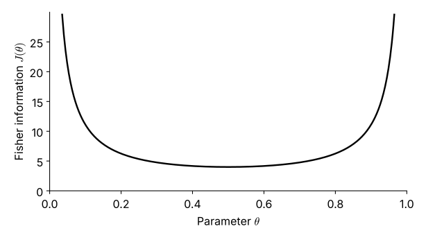
\[\begin{aligned} J(\theta) &= \mathbb{E}_{x_i \in \mathcal{X}} \left[ \left( \frac{\partial}{\partial \theta} \ln f(x_i;\theta) \right)^2 \right] \\ &= \mathbb{E}_{x_i \in \mathcal{X}} \left[ \left( \frac{\partial}{\partial \theta} \ln \theta^{x_i}(1 - \theta)^{1-x_i} \right)^2 \right] \\ &= \mathbb{E}_{x_i \in \mathcal{X}} \left[ \left( \frac{\partial}{\partial \theta} \Big[ x_i \ln \theta + (1-x_i) \ln (1-\theta) \Big] \right)^2 \right] \\ &= \mathbb{E}_{x_i \in \mathcal{X}} \left[ \left( \frac{x_i}{\theta} - \frac{1-x_i}{1-\theta} \right)^2 \right] \\ &= \mathbb{E}_{x_i \in \mathcal{X}} \left[ \left( \frac{x_i - \theta}{\theta (1-\theta)} \right)^2 \right] \\ &= \theta \frac{(1-\theta)^2}{\theta^2 (1-\theta)^2} + (1-\theta) \frac{(-\theta)^2}{\theta^2 (1-\theta)^2} \\ &= \frac{1}{\theta (1-\theta)}. \end{aligned}\]This is the unit Fisher information for Bernoulli trials, which is visualized in the figure below. Intuitively, when the parameter \(\theta\) is close to 0 or 1, even one single trial is very informative about \(\theta.\) In contrast, when \(\theta\) is close to 0.5, the result of only one trial is not very informative.
Multiple Bernoulli trials and sufficient statistic. According to Eq. (2), the Fisher information about the parameter \(\theta\) within \(n\) i.i.d. trials is
\[J_{X^n}(\theta) = n J_X(\theta) = \frac{n}{\theta (1-\theta)}.\]Now let’s consider a summary statistic \(Y\), which is the number of 1s within \(n\) trials, \(Y = \sum_{i=1}^n X_i\), and it follows the Binomial distribution
\[f(y; \theta) = \binom{n}{y} \theta^y (1-\theta)^{n-y}, \quad \text{where } y \in \mathcal{Y} = \{0, 1, \dots, n\}.\]We can calculate the Fisher information in \(Y\) about \(\theta\) using the Binomial distribution. The result is \(J_Y(\theta) = \frac{n}{\theta (1-\theta)}\), which is the same as the Fisher information in the raw data sequence, \(J_Y(\theta) = J_{X^n}(\theta).\) Therefore, \(Y\) and \(X^n\) provide the same amount of information about \(\theta.\) \(Y\) is therefore a sufficient statistic of the raw data \(X^n,\) since no information is lost about \(\theta.\)